Level 1 CFA® Exam:
IS-LM Model & Other Topics
To explain this relationship among savings, investments, the fiscal balance, and the trade balance, we need to compare the income and expenditure approaches to calculating GDP.
In the expenditure approach:
\(GDP=C+I+G+(X-M)\)
In the income approach:
\(GDP=C+S+T\)
Where:
- C - household consumption,
- S - savings of households and companies,
- T - net taxes (direct and indirect taxes minus transfer payments),
- I – investments,
- G - government spending,
- X – exports,
- M - imports.
Because in an economy total expenditure equals aggregate income, therefore:
\(C+I+G+(X-M)=C+S+T\)
Thus:
Fiscal Balance
In the formula, the fiscal balance is represented as \((G-T)\), so it's the difference between government spending and net taxes.
(...)
Trade Balance
\((X-M)\), that is exports minus imports, is called the trade balance.
If:
- \((X-M) > 0\) >> trade surplus (exports receipts exceed imports expenditure),
- \((X-M) < 0\) >> trade deficit (imports expenditure exceed exports receipts),
\((X-M)=(S-I)-(G-T)\)
Marginal Propensity to Consume (MPC) vs Marginal Propensity to Save (MPS)
star content check off when doneHouseholds can either consume their disposable income or save it.
The proportion of the additional unit of disposable income that is spent is called marginal propensity to consume (MPC).
The proportion of the additional unit of disposable income that is saved is called marginal propensity to save (MPS).
The disposable income of John Gates has raised from USD 3,000 to USD 3,600. John has decided to spend USD 400 of additional income. What is the value of MPC and MPS?
(...)
The IS-LM model is a tool that tells us about the relationship between the goods and services market and the money market. The acronym in the name of the model stands for Investment Saving–Liquidity Preference Money Supply.
In the model, an economy is divided into two markets:
- the goods and services market, and
- the money market.
The IS-LM model focuses on the short-run macroeconomic equilibrium in both markets and the correlation between them.
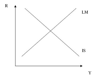
In the graph, the X-axis is denoted by Y, which stands for aggregate output, and the Y-axis is denoted by R, which stands for interest rate. There are also two curves, IS and LM, that intersect.
The intersection of the IS and LM curves demonstrates the level of GDP and the interest rate at which equilibrium is achieved in both the goods and services market and the money market.
When there is equilibrium in both markets, aggregated income equals planned expenditures in the goods and services market and money demand equals money supply in the money market.
IS curve:
- is a function of equilibrium in the goods and services market,
- presents combinations of GDP and interest rates at which the market is in equilibrium,
- equilibrium occurs when: aggregated income = expenditures,
- is negatively sloped.
Movement along the IS curve is typically a consequence of a change in the interest rate:
(...)
LM curve:
- is a function of equilibrium in the money market,
- presents combinations of GDP and interest rates at which the money market is in equilibrium,
- equilibrium occurs when: money demand = money supply,
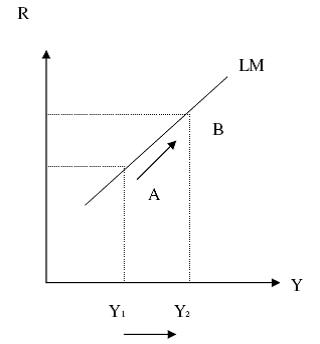
- is positively sloped.
Movement along the LM curve is usually the outcome of a change in GDP. In the money market, the relationship between income and the interest rate is positive. So, when output goes up, so does the transaction demand for money (because more money is necessary to carry out a greater number of transactions). At a given constant level of supply of money, an increase in demand makes market participants withdraw their savings from banks, and the price of money, that is the interest rate, goes up. As you can see, an increase in output from \(Y_1\) to \(Y_2\) results in an increase in the interest rate form \(R_1\) to \(R_2\).
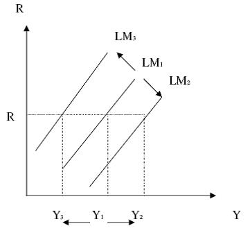
All else equal, a shift of the LM curve may be a result of an increase in money supply (a consequence of an expansionary monetary policy) or a decrease in money supply (if monetary policy is contractionary).
If the money supply goes up, the LM curve moves to the right from \(LM_1\) to \(LM_2\) and output increases from \(Y_1\) to \(Y_2\) with a given value of interest rate. Conversely, if the money supply goes down, the LM curve moves to the left to \(LM_3\) and output also moves to the left to \(Y_3\).
The intersection of the IS and LM curves demonstrates the level of GDP and the interest rate at which equilibrium is achieved in both the goods and services market and the money market.
The intersections of the IS curve and the LM curve for different levels of money supply delineate the aggregate demand curve (AD curve).
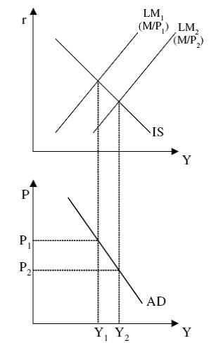
All else equal, the AD curve reflects the negative relationship between GDP and the price level.
A shift of the AD curve may be caused by:
(...)
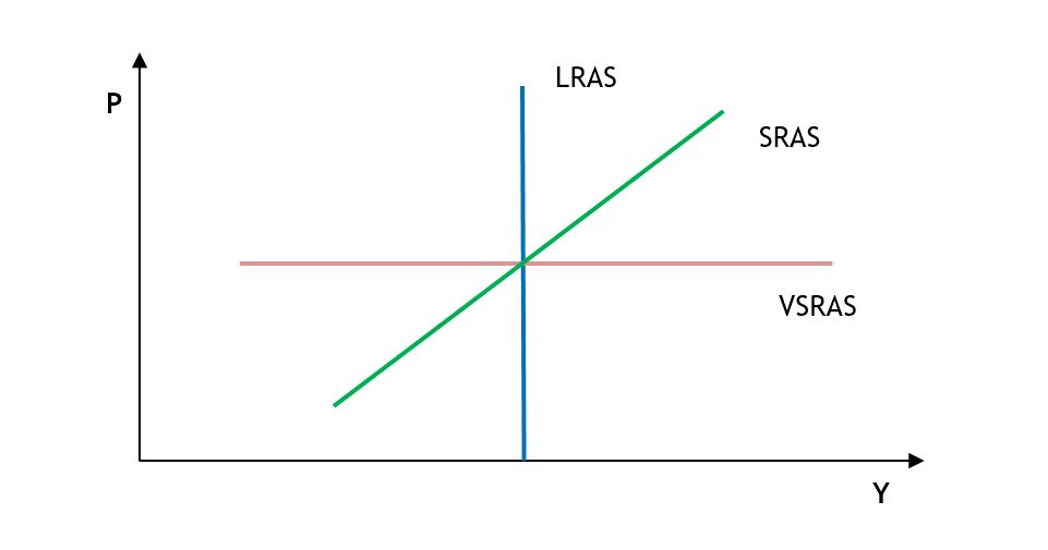
The aggregate supply curve (AS curve) illustrates a positive correlation between the level of prices and the aggregate output of an economy.
We distinguish:
- very-short-run aggregate supply (VSRAS) curve,
- short-run aggregate supply (SRAS) curve,
- long-run aggregate supply (LRAS) curve.
The slope of the AS curve depends on the time period:
- in a very short run >> the AS curve is horizontal,
- in the short run >> the AS curve is upward sloping. Provided that prices of factors of production are held constant, higher prices of goods and services result in increased output. It means that in the short run some of the prices are assumed to be sticky.
- in the long run >> the AS curve is vertical. It means that the LRAS curve is perfectly inflexible and simply represents the level of potential output. It is because the prices of factors of production adjust to changes in prices of goods and services in the long run. In other words, it means that in the long run all prices are flexible.
Shift of SRAS Curve
A shift of the SRAS curve may be caused by:
(...)
Shift of LRAS Curve
The LRAS curve shifts to the right when there is technological progress or an increase in productivity or a greater quantity of factors of production, like labor or capital.

- If there is a fiscal deficit, then at least one of two things occurs: the private sector saves more than invests and the country runs a trade deficit.
- The proportion of the additional unit of disposable income that is spent is called marginal propensity to consume (MPC).
- The proportion of the additional unit of disposable income that is saved is called marginal propensity to save (MPS).
- The IS-LM model is a tool that tells us about the relationship between the goods and services market and the money market.
- The intersection of the IS and LM curves demonstrates the level of GDP and the interest rate at which equilibrium is achieved in both the goods and services market and the money market.
- Movement along the IS curve is typically a consequence of a change in the interest rate.
- The government's contractionary fiscal policy, that is a policy involving a reduction in government expenditure or an increase in taxes, will result in a downward shift of the IS curve.
- Movement along the LM curve is usually the outcome of a change in GDP.
- A shift of the LM curve may be a result of an increase in the money supply or a decrease in the money supply.
- The aggregate demand curve (AD curve) can be derived from the intersection points of the IS and LM curves.
- The aggregate supply curve (AS curve) illustrates a positive correlation between the level of prices and the aggregate output of an economy.
- We distinguish: the very-short-run aggregate supply (VSRAS) curve, short-run aggregate supply (SRAS) curve, and long-run aggregate supply (LRAS) curve.