Level 1 CFA® Exam:
Continuous Uniform Distribution & Monte Carlo Simulation
Introduction to Continuous Uniform Distribution
In the last two lessons, we discussed some issues related to a discrete random variable and two of its possible distributions, namely:
- the discrete uniform distribution (e.g. rolling a dice), and
- the binomial distribution (e.g. flipping a coin multiple times).
In this lesson, we discuss the continuous uniform distribution, which is very similar to the discrete uniform distribution. The difference is that for the continuous uniform distribution we use a continuous random variable instead of a discrete one.
A continuous random variable can take any values from a specified range. The probability function of a continuous random variable is called probability density function, or simply density. Note, that when we're dealing with a continuous random variable, the probability that the random variable takes on a precisely specified value is always 0. We can, however, calculate the probability that a random variable takes on a value between two different values A and B. The probability that the random variable takes on a value between A and B equals the area under the graph of the density function between points A and B.
The simplest example of a continuous distribution is the continuous uniform distribution. It's used for example in Monte Carlo simulation, which we're going to discuss later on.
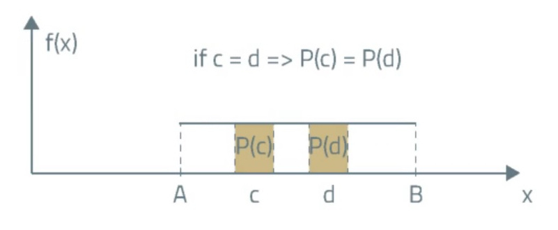
As you can see on the graph of the density function of the continuous uniform distribution, for any two intervals with the same length the probability that the random variable takes on the value from any of these two intervals is the same. It is because the density function of the continuous uniform distribution is parallel to the X-axis.
So, the density function for a uniform random variable takes the following form:
In this formula 'A' is the lower limit of the interval and 'B' is the upper limit of the interval.
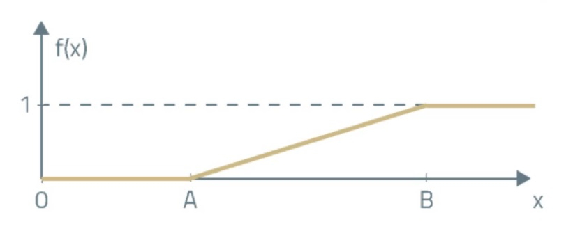
On the other hand, the cumulative distribution function for a continuous uniform distribution is expressed as follows:
Suppose we're considering a random variable that follows a continuous uniform distribution extending over the interval of [0, 10]:
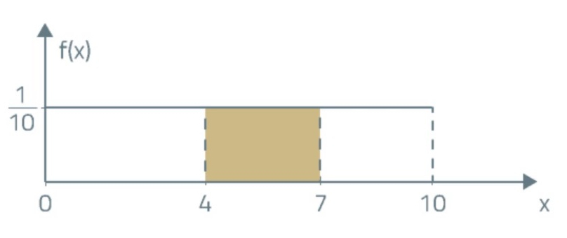
- What's the probability that the variable takes a value between 4 and 7?
- What is the probability that the random variable will be exactly equal to 7?
(...)
The expected net profit of We are the Winners, Inc. is described by continuous uniform distribution and its upper limit equals USD 10.4 million. Additionally, you find out that the probability that the expected net profit will be greater than USD 5.2 million is 35%. What are the lower limit and the range of the expected net profit for the company?
(...)

Monte Carlo simulation is used to simulate complex processes whose results are hard to predict using analytical methods. This method is based on repeated trials in which you draw predefined parameters affecting, for example, the price of a security.
Before we start simulation it is necessary to determine the probability distributions for the parameters used in the simulation. Trials are repeated several thousand times and every single time a valuation is conducted. Finally, the expected value of the security is calculated.
Monte Carlo is used among other things to:
- Value securities, including complex derivatives and strategies that involve them.
- Simulate trading and investment strategies.
- Estimate Value at Risk (aka. VAR).
- Value assets with distributions other than normal.
However, there may be some limitations to this method because:
- Monte Carlo simulation is a complex and laborious process.
- The simulation results are only as good as the assumptions that you make.
Some people also argue that, as a statistical method, it doesn’t allow you to examine some problems as thoroughly as analytical methods do.
(...)
Level 1 CFA Exam Takeaways: Continuous Uniform Distribution & Monte Carlo Simulation
star content check off when done- A continuous random variable can take any values from a specified range.
- The probability function of a continuous random variable is called the probability density function.
- The density function of the continuous uniform distribution, for any two intervals with the same length the probability that the random variable takes on the value from any of these two intervals, is the same.
- Monte Carlo simulation is used to simulate complex processes whose results are hard to predict using analytical methods.
- The Monte Carlo simulation results are only as good as the assumptions that you make.
- A big disadvantage of historical simulation are general doubts as to whether the future price of assets can be estimated using historical data.