Level 1 CFA® Exam:
Downside Deviation, Coefficient of Variation & Correlation
If we think about the variance and standard deviation as a measure of risk, we should notice that they measure the dispersion of observations both below and above the mean. However, investors are generally afraid of incurring a loss on the investment and are satisfied when they have a gain. Therefore, instead of using standard deviation as a measure of risk, we can use the so-called target semideviation as a measure of risk.
Target semideviation (aka. target downside deviation) is used by investors as a measure of risk instead of, e.g., standard deviation.
Target semideviation has 2 interesting features. First of all, it concentrates only on the part of the results that are low, hence semidevation instead of deviation in the name. Secondly, we don’t calculate it for the results that are below the mean (although we could) but we can choose any target that interests us, hence target in the name.
For example, if someone invests in a low-risk portfolio, they can choose the risk-free interest rate as the target and calculate the dispersion below the target. The higher the value of the target semideviation, the higher the risk of the portfolio and potential loss.
Here’s the formula for the sample target semideviation to be used in your level 1 CFA exam:
The table below presents historical returns on a portfolio. An investor wants to preserve his capital and is afraid of incurring any loss. What target should he choose? What is the value of the target semideviation?
| Year | Rate of return (%) |
|---|---|
| 2014 | 4 |
| 2015 | 15 |
| 2016 | 31 |
| 2017 | 22 |
| 2018 | -19 |
| 2019 | -9 |
| 2020 | 12 |
| 2021 | 4 |
| 2022 | -1 |
(...)
The standard deviation is expressed in the same units of measurement as observations, which is to the advantage of an analyst, as it makes its interpretation easier. However, if we want to compare the dispersion of two datasets, the standard deviation may not be the right measure.
For example, let’s assume we want to analyze and compare the value of the sales of a small company and a large one. Suppose the standard deviation of the monthly sales of the large company equals USD 500,000, and of the small one equals USD 10,000. Which of the two companies is characterized by the greater dispersion of monthly sales?
We might wrongly assume that the sales of the large company are more dispersed than those of the small one, as the standard deviation for the large one is greater. However, standard deviation alone is not enough to arrive at a reliable comparison. To compare sales volatility in the two companies, we need a relative measure of dispersion to standardize the dispersion of observations. One such measure is the coefficient of variation.
Coefficient of variation (CV) – a relative statistical measure of data dispersion expressed as a ratio of the standard deviation of a sample and sample mean.
The coefficient of variation is expressed with the following formula:
The coefficient of variation is expressed as a percentage or multiple. The greater the coefficient of variation, the greater the risk per unit of the arithmetic mean. Back to our example about two companies: the small one, and the large one. If we wanted to calculate the coefficient of variation first, we would have to compute the average sales in the two companies in the examined period. Then we need to divide the standard deviation by the average sales for both companies and compare the obtained results. The company whose coefficient of variation is greater is characterized by greater volatility of sales.
We have the following data on the annual returns of a fund:
| Year | Rate of return (%) |
|---|---|
| 2014 | 4 |
| 2015 | 15 |
| 2016 | 31 |
| 2017 | 22 |
| 2018 | -19 |
| 2019 | -9 |
| 2020 | 12 |
| 2021 | 4 |
| 2022 | -1 |
Calculate and interpret the coefficient of variation based on the data.
(...)
What else should you know about the coefficient of variation?
The coefficient of variation can be used not only to compare the dispersion of datasets with very different arithmetic means, like in the case of the large company and the small one, but also if the observations in the datasets are expressed with different units of measurement. It is because the coefficient of variation is always expressed as a percentage (or multiple), no matter what the unit of measurement of the dataset is.
Remember also that the greater the coefficient of variation, the greater the risk per unit of the arithmetic mean. So, if – for example – you compare the performance of two investment funds, the fund with the greater coefficient of variation will be characterized by greater risk.

Sample covariance is a statistical relationship that measures the extent to which two variables move in the same direction. A positive covariance, that is a covariance greater than 0, means that if the value of one variable goes up, the value of the other variable will also go up, and vice versa. If the value of one variable goes down, the value of the other variable will also go down. A negative covariance, on the other hand, means that the values of the variables move in opposite directions. Unfortunately, these are the only conclusions we can draw based on covariance.
(...)
A scatter plot is a graph illustrating the relationships between two variables. The points on the graph are marked based on two coordinates – the values of the variables (for example the values of Variable A are marked on the X-axis and the values of Variable B – on the Y-axis). If you have a look at the graph, you'll see four example relationships between the two variables A and B.
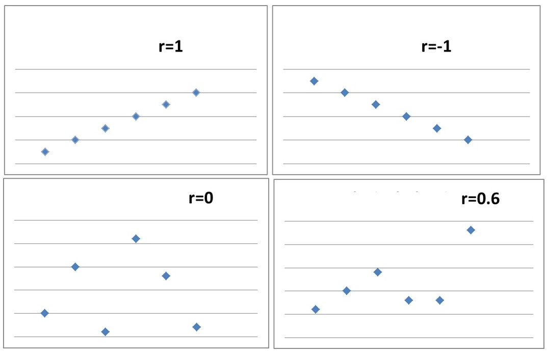
In the case of a perfect positive or negative correlation, the points on the graph plot a straight line. If we're dealing with a zero correlation, the points are randomly scattered without a discernible pattern. The correlation coefficient equal to 0.6 indicates a positive correlation between variables, but the points on the graph don’t plot a straight line like in the case of the correlation coefficient equal to 1.
Sample covariance between two variables is computed using this formula:
You're probably wondering how to interpret covariance. As we said before, there is no unambiguous interpretation of covariance for a unit of measurement. The values of covariance are unbounded. So, to easily interpret the relationship, we use the correlation coefficient.
We can say that the correlation coefficient is a standardized covariance, so the correlation coefficient is a value within the interval between (- 1) and (+ 1). The correlation coefficient can be computed using this formula:
The correlation coefficient equals covariance divided by the product of the sample standard deviations.
Let's take a look at an example.
Suppose the correlation between two variables equals 0.7. The variance of random variable A is 23.254 and the variance of random variable B is 150.567. Compute the covariance.
(...)
What we understand as a perfect positive correlation is a correlation coefficient of \(\rho=1\). \(\rho=-1\) indicates a perfect negative correlation. Unsurprisingly, a zero correlation is characterized by a correlation coefficient of \(\rho=0\). Now, any correlation coefficient ranging from 0 to 1 indicates a positive correlation, whereas the correlation coefficient between 0 and minus 1 shows a negative correlation.
One example of a situation when correlation analysis can be useful is when we want to check if a portfolio manager who invests in large companies (that is ones with a major capitalization) is leaning more towards growing companies or high-value companies.
Correlation analysis allows us also to examine how much returns earned by the investment fund are correlated with the returns on an index. When we know that, we can decide if it pays more to invest in the fund that charges management fees or invest passively in the index for example using an ETF.
You must remember that most statistical and econometric tools have limitations concerning their application. So it is the case with correlation.
The major limitations in the use of correlation analysis are:
- nonlinear relations,
- spurious correlations,
- and outliers.
(...)
Level 1 CFA Exam Takeaways: Downside Deviation, Coefficient of Variation & Correlation
star content check off when done- Target semideviation (aka. target downside deviation) is used by investors as a measure of risk instead of, e.g., standard deviation.
- The coefficient of variation (CV) is a relative statistical measure of data dispersion expressed as a ratio of the standard deviation of a sample and sample mean.
- The greater the coefficient of variation, the greater the risk per unit of the arithmetic mean.
- The sample covariance is a statistical relationship that measures the extent to which two variables move in the same direction.
- A scatter plot is a graph illustrating the relationships between two variables.
- The correlation coefficient measures linear relationships between variables. The correlation coefficient is a standardized covariance, so the correlation coefficient is a value within the interval between (- 1) and (+ 1).
- The major limitations in the use of correlation analysis are nonlinear relations, spurious correlations, and outliers.
- Outliers are extreme observations, that is observations extremely different from the majority of observations for a variable.
- A spurious correlation is when analysis shows a relationship between variables when there is actually none.