Level 1 CFA® Exam:
Capital Asset Pricing Model (CAPM)
In this lesson, we're going to discuss the Capital Asset Pricing Model (CAPM). This model is particularly appreciated in today's finance and used by analysts from across the world.
What are the key characteristics of the model? On the one hand, it is simple and intuitive, but it involves many assumptions that often do not stand up to reality. It was introduced independently by Treynor, Sharpe, Lintner, and Mossin who drew on Harry Markowitz's earlier work. The model shows the relationship between the risk and the expected return.
CAPM is based on two equations. The first one is the capital market line (CML) expressed with this formula:
Just to remind you, this equation is only true for efficient portfolios.
The other equation is the security market line (SML) which shows the relationship between the systematic risk and the expected return on an asset or a portfolio of assets:
The model is based on 6 main assumptions:
- Investors are risk-averse, utility-maximizing, rational individuals.
- Markets are frictionless, including no transaction costs and no taxes.
- Investors plan for the same single holding period.
- All investors have homogeneous expectations.
- All investments are infinitely divisible.
- Investors cannot influence prices.
Investors are risk-averse, utility-maximizing, rational individuals.
Remember that a risk-averse investor will expect to be compensated for accepting higher risk. Note that risk aversion does not mean that all investors will accept the same level of risk.
Utility maximization simply means that an investor prefers to have more wealth than less.
The first two postulates are generally true in the real world. What is questioned is the rationality of investors. In practice, investors are often irrational as their decision-making may be affected by different subjective factors even though they use the same information.
Markets are frictionless, including no transaction costs and no taxes.
Friction costs are costs that arise from the difference between buying and selling prices and are connected with market liquidity. The assumption of no transaction costs and no taxes is present in many models. Depending on how high friction costs, transaction costs, and taxes are, they may affect conclusions drawn from the CAPM to a larger or smaller extent.
Investors plan for the same single holding period.
All investors will have the same single holding period. This assumption is supposed to simplify the model. The CAPM also served as the basis for the multi-period capital asset pricing model, but we will not focus on it.
(...)
Now, let's talk about the capital market line and the security market line in more detail.
Let’s focus on the essence of the CAPM. Just as we've just mentioned, it's based on two equations. The first one is the capital market line expressed with the formula:
Recall that this equation is only true for efficient portfolios. So, it allows us to estimate whether a given portfolio is efficient.
The second equation is the security market line expressed with this formula:
The SML applies to all portfolios, including portfolios that comprise only a single security.
The essence of the CAPM is a market portfolio, the same for all investors, and the relationships obtained from the CML and the SML.
Relationships Obtained from CML & SML
The first relationship stems from the CML and concerns efficient portfolios. It’s about the fact that the rate of return on an efficient portfolio is the sum of the risk-free rate (which may be seen as the price for postponing an investor's consumption) and the expected market return less risk-free rate divided by the standard deviation of market returns and multiplied by the portfolio total risk.
In accordance with the CML, the rate of return may be expressed as the time price and risk price multiplied by the total risk.
The second relationship for the CAPM stems from the SML and shows the rate of return as the sum of the risk-free rate (just as in the CML equation) and the risk price multiplied by the amount of risk. However, in this case, we take into consideration only the systematic risk, which means that we have a product of the amount of systematic risk measured with beta and the rate of return on the market portfolio less a risk-free rate of return (that is the so-called market risk premium).
The market portfolio return is 12%. The risk-free rate is 3.5%. The beta of an ABC stock is 1.15. Calculate the expected rate of return.
(...)
If you know that according to the CAPM the expected return on an LPP stock is 14%, the risk-free rate is 1.5% and the beta of LPP is estimated at 1.76, calculate the market risk premium and market portfolio return.
(...)
(...)
The graphs below show the relationship between the SML and the CML.
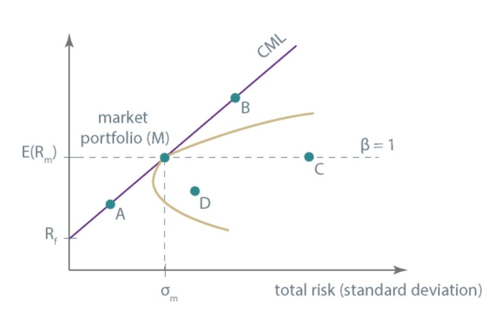
On the capital market line lie portfolios A, B, and the market portfolio M. Portfolio A includes risk-free assets and the market portfolio and it is an efficient portfolio. Portfolio B is also an efficient portfolio, but it is a leveraged one (debt was incurred at the risk-free rate to buy more market portfolio). Portfolios C and D are inefficient because they lie below the efficient frontier.
Portfolio C has beta equal to 1, so the expected return will equal the expected market portfolio return.
Even though portfolios C and D are inefficient, they can lie on the security market line because the SML relates to market risk, and the CML to total risk. It is visible for portfolio C. Its beta is 1, the same as for the market portfolio, but because the market portfolio is well-diversified, unlike portfolio C, its total risk is lower. Portfolio C is not efficient because, as we claimed in our previous lessons, an investor shouldn’t expect to be compensated for unsystematic risk.
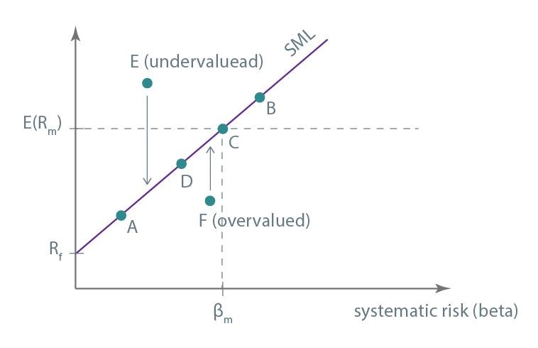
Now, let's illustrate the most important applications of the CAPM. In the graph presenting the SML, you could see that portfolios A, B, C, and D are properly valued. They lie on the SML, so the expected rate of return is the same as in the case of most of the portfolios with the same beta. Two portfolios, E and F, do not lie on the security market line, so we can conclude that they are not accurately valued.
Portfolio E has a higher expected rate of return for a given market risk than it would follow from the SML. Therefore, it is an undervalued portfolio which is a catch for investors. The CAPM is supposed to be a balanced model. Increased demand for portfolio E causes a rise in its price and, in consequence, a decrease in return to the level following from the SML.
Portfolio F is overvalued, which means that the expected rate of return on the portfolio is lower than you would expect from the SML. The fact that the portfolio is overvalued will make investors sell it, which will bring about a decrease in its price and ultimately an increase in the expected rate of return to the level you would expect from the SML.
This way, under the CAPM, the balance on capital markets is achieved. The issue we’ve just discussed is one of the ways of selecting securities for a portfolio. An investor compares an expected rate of return estimated with the aid of other methods, say fundamental analysis, with the rate of return obtained from the SML and invests in undervalued portfolios, for example in portfolio E.
The risk-free rate is 2%. The market risk premium is 7%. Analysts estimate the return on stock A at 7.5%, and on stock B at 11%. The beta of A is 0.73 and of B is 1.3. Which stocks should be selected for the portfolio?
(...)
Apart from such purposes as selecting undervalued and overvalued securities or estimating rates of return, the CAPM is widely applied in evaluating the performance of investments that have already been made. Among many things, it can be used to evaluate the work of a fund manager. Because every investment carries some risk, performance measures relate to risk and the rate of return on investment.
To understand performance measures better, let’s analyze 4 ratios:
- Sharpe ratio,
- Treynor ratio,
- Jensen’s Alpha, and
- M-Squared.
Sharpe Ratio
The Sharpe ratio uses the total risk measured with the standard deviation of the portfolio and has the formula that looks like this:
The Sharpe ratio is equal to the excess return of the portfolio divided by the total risk.
The ratio is compared with the ratios of other portfolios. A portfolio with a higher Sharpe ratio has a better performance as it gets a higher return per unit of total risk.
Treynor Ratio
The Treynor ratio also shows excess portfolio return over the risk-free rate but this time it is per unit of systematic risk measured with the beta of the portfolio.
Just as in the case of the Sharpe ratio, the higher the Treynor ratio, the better the management of the portfolio.
Note that if we evaluate well-diversified portfolios, their ranking will be the same for both the Sharpe and Treynor ratios. Additionally, you should bear in mind that the Treynor ratio can only be applied to well-diversified portfolios, that is portfolios that have only the systematic risk, because –to estimate the risk – we need beta, which is in fact a measure of systematic risk.
Now, imagine a scenario in which you have two portfolios: A and B. Portfolio A has a higher Treynor ratio than portfolio B, but portfolio A has nonsystematic risk, which means it is not a well-diversified portfolio. There is a possibility that if we consider the total risk of both portfolios, portfolio B would be liable to perform better. For this scenario, to get a reliable result, you should calculate the Sharpe ratio, which uses total risk measured with the standard deviation of the rate of return.
Assume you have the data given in the table:
| Portfolio | Portfolio return (%) | \(\sigma\) | \(\beta\) |
|---|---|---|---|
| A | 10 | 12 | 1.4 |
| B | 15 | 19 | 2.3 |
| C | 5 | 4 | 0.36 |
The risk-free rate is 3%. Which portfolio was better managed if we use the Sharpe ratio, and which if we apply the Treynor ratio?
(...)
Jensen’s Alpha
Using Jensen's alpha, we calculate the difference between the actual portfolio return and the return of the hypothetical portfolio lying on the SML. The formula for Jensen's alpha looks as follows:
If Jensen's alpha is positive, it means that the portfolio earned more than the security market line (SML) shows, which proves that the portfolio is managed efficiently. If Jensen's alpha is negative, the portfolio is managed inefficiently.
M-Squared
The last ratio we are going to discuss is the M-Squared. It is the most recent measure out of the ones we’ve mentioned so far. It was developed by an American economist Franco Modigliani and his granddaughter, Leah. This measure was derived from the Sharpe ratio and uses total risk. So-called M-Squared alpha is expressed with a formula presented below:
Thanks to multiplying \(R_p-R_f\) by \(\frac{\sigma_m}{\sigma_p}\) we reduce the excess return on the portfolio to the rate of return on the portfolio with the risk equal to the risk of the market portfolio. Next, we compare this changed return with the actual excess market portfolio return.
If we obtain a positive value, it means that the portfolio was managed efficiently and earned more than the respective investment in the market portfolio. If we obtain a negative value, it means that the portfolio was managed inefficiently and earned less than the respective investment in the market portfolio.
M-squared alpha gives us rankings that are identical to those of the Sharpe ratio. However, it is easier to interpret, because it is expressed as a percentage and it is an absolute measure just like Jensen's alpha and unlike the Sharpe and Treynor ratios.
(...)
Also, there are more practical versions of CAMP like Fama, French, and Carhart's four-factor model:

- CAPM is based on two equations: capital market line (CML) and security market line (SML).
- CAPM is based on 6 main assumptions: (1) Investors are risk-averse, utility-maximizing, rational individuals. (2) Markets are frictionless, including no transaction costs and no taxes. (3) Investors plan for the same single holding period. (4) All investors have homogeneous expectations. (5) All investments are infinitely divisible. (6) Investors cannot influence prices.
- In the case of SML we take into consideration only the systematic risk.
- If beta is between 0 and 1, then the rate of return on the investment is higher than the risk-free rate and lower than the market portfolio return.
- Overvalued portfolios are below the SML line, whereas undervalued portfolios can be found above the SML line.
- The Sharpe ratio uses the total risk measured with the standard deviation of the portfolio.
- The Treynor ratio shows excess portfolio return over the risk-free rate per unit of systematic risk measured with the beta.
- Using Jensen's alpha, we calculate the difference between the actual portfolio return and the return of the hypothetical portfolio lying on the SML.
- M-squared alpha gives us rankings that are identical to those of the Sharpe ratio.
- The arbitrage pricing theory (APT) is a multi-factor model with 2 assumptions: (1) the law of one price and (2) the homogeneity in investor expectations.