Level 1 CFA® Exam:
Lognormal Distribution
Lognormal Distribution in CFA Exam: Definition, Properties, Formulas
star content check off when doneIn one of the previous lessons, we discussed the normal distribution. Another distribution that is widely used in finance is the lognormal distribution. It’s used, among others, in the Black-Scholes-Merton option pricing model. So, let’s explain how this distribution is constructed.
If X is a random variable that follows a normal distribution, then \(e^X\) is a random variable that follows a lognormal distribution. \(e\) stands for Euler’s number named after Leonhard Euler – a Swiss mathematician. \(e\) is approximately equal to 2.718.
On the other hand, when X is a random variable following a lognormal distribution, then \(lnX\) is a normally distributed random variable. The natural logarithm (\(ln\)) is the logarithm to the base \(e\).
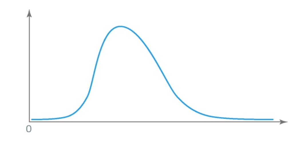
The lognormal distribution has the following properties:
- It is skewed to the right.
- On the left, it is bounded by 0.
- It is described by two parameters of associated normal distribution, namely the mean and variance.
(...)
A random variable X is normally distributed with the mean equal to 10% and the standard deviation equal to 25%. What is the mean and variance of the associated lognormal random variable?
A random variable X is normally distributed with the mean equal to 10% and the standard deviation equal to 25%. What is the mean and variance of the associated lognormal random variable?
To calculate the mean of the lognormal random variable, we have to find the variance of the normally distributed random variable first.
The variance equals the standard deviation squared, that is 25% squared, which gives us 0.0625.
So, the mean of the lognormal random variable equals:
\(\text{mean}=e^{0.1+0.5\times0.0625}=1.1403\)
The variance of the lognormal distribution is:
\(\text{variance}=e^{2\times\mu+\sigma^2}\times{(e^{\sigma^2}-1)}= e^{2\times0.1+0.0625}\times{(e^{0.0625}-1)}=0.0839\)
Here are 3 formulas for continuously compounded returns that you can use in your level 1 CFA exam:
The price of a stock at the beginning of a year is equal to USD 56 and at the end of the year equals USD 70. What is the holding period return and continuously compounded return for this year?
(...)
Very often securities valuation models assume that continuously compounded returns of securities are normally distributed. Based on this assumption, it can be proved that prices of securities are lognormally distributed. Thanks to it, we can use the lognormal distribution to model the probability distribution of security prices, which is very useful for modeling prices of securities.
You should also remember that even if continuously compounded returns of securities are not exactly normally distributed, then according to the central limit theorem, security prices can be well described by the lognormal distribution.

- If X is a random variable that follows a normal distribution, then \(e^X\) is a random variable that follows a lognormal distribution.
- The lognormal distribution has the following properties: (1) It is skewed to the right, (2) on the left, it is bounded by 0, and (3) it is described by two parameters of associated normal distribution, namely the mean and variance.
- Lognormal distribution can be used for modeling prices and normal distribution can be used for modeling returns.